Divide-and-conquer|分治算法

Kevin 吴嘉文大约 6 分钟

Divide-and-conquer is easy to understand, but hard to create. This article will discuss the key for proofing Divide-and-conquer as well as some ideas for solving a new problem using divide-and-conquer based on these 4 topics: Merge Sort, Quick Sort, Hanoi and Closet Point

Merge Sort

Merge Sort is the first example for divide and conquer algorithms examples in CLRS. Hence, it might consider as the easiest divide and conquer algorithm in the book. Time complexity $O(nlgn)$

Main idea of merge sort

In merge step, when 2 sorted sequences are combined together, the output sequence will be well sorted. Therefore, under divide-and-conquer, the initial sequence will be divided until base units, which is single number in this case. Single number is sorted sequence, hence all the sequence in the following step will be sorted well.

There are 3 key component of this case:

Initialization

Personally, the divide-and-conquer might consider as 2 step, divide and merge. In divide step, the input is initial sequence. The algorithm should consider this length of sequence is odd or even. In merge step, the input is a set of single number.

Maintenance

In divide step, maintenance is just divide input sequence into 2 sequence with same length. When merge, we need Merge algorithm to combine 2 sorted sequences.

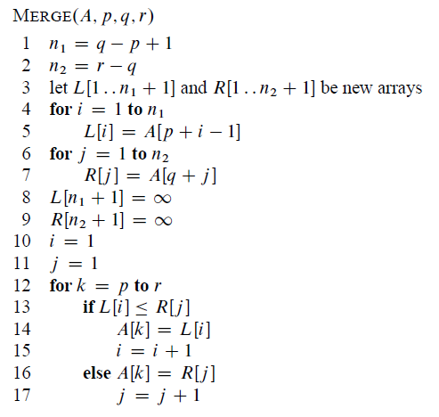
(picture source: CLRS p31) A is the initial array, p, q are the index of the begin of two input sequence that we discuss above. r is the index of end of Right hand side array.

Termination

When divide, the algorithm end at unit number. When merge, the algorithm ends at a sorted sequence.

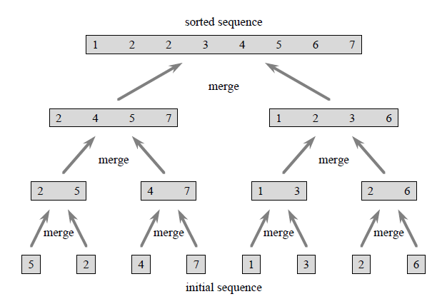
Of course, you might want to use math to proof the above 3 components if necessary. The difficult part of merge sort is dealing with odd and even length of sequence well.

Following is the code in python.

def merge_sort(A, lower, upper):
    compare_count, assign_count = 0, 0
    if lower < upper:
        mid = (lower + upper) // 2
        cc, ac = merge_sort(A, lower, mid)
        compare_count += cc
        assign_count += ac
        cc, ac = merge_sort(A, mid + 1, upper)
        compare_count += cc
        assign_count += ac
        tmpL = [0] * (mid - lower + 2)
        for i in range(0, mid - lower + 1):
            tmpL[i] = A[i+lower]
        tmpL[mid - lower + 1] = float('inf')
        tmpR = [0] * (upper - mid + 1)
        for j in range(0, upper - mid):
            tmpR[j] = A[j+mid+1]
        tmpR[upper - mid] = float('inf')
        i, j = 0, 0
        for k in range(lower, upper + 1):
            if tmpL[i] <= tmpR[j]:
                A[k] = tmpL[i]
                assign_count += 1
                i += 1
            else:
                A[k] = tmpR[j]
                assign_count += 1
                j += 1
            compare_count += 1
        del tmpL, tmpR
    return compare_count, assign_count

QuickSort

Main idea of QuickSort

Step 1: pick a number as x, in input sequence, put those number larger then x into right hand side of x. Those numbers smaller than x will be at the left hand side of x.

Step 2: Repeat Step 1 on both right hand side sequence and left hand side sequence until the length of sequence is 1.

The following is an example, the number picked is 4.

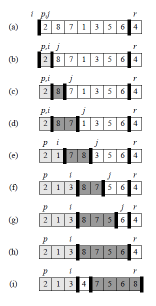
(picture source: CLRS P172)

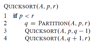
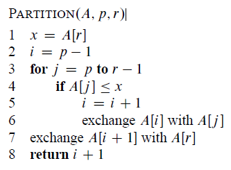
The key point for quicksort is partition step. It is important for you to pick some numbers, and go through the partition algorithm step by step if you want to fully understand why it is correct . When building a binary tree, you might see similar steps as partition.

Time Complexity

The partition step takes $O(n)$ .

The worst-case time complexity could be $O(n^2)$ , when all the problem was divided into subproblems with n-1 items and 0 item.

\begin{aligned} T(n) &=T(n-1)+T(0)+\Theta(n) \mid \\ &=T(n-1)+\Theta(n) \end{aligned}

The best-case is we always pick the number in the middle, which gives a time complexity of $O(nlgn)$

\begin{aligned} T(n) &=2T(n/2)+\Theta(n) \end{aligned}

Even we divide the sequence with a 9-to-1 proportion. The time complexity is still $O(nlgn)$

\begin{aligned} T(n)&=T(9n/10)+T(n/10)+\Theta(n) \end{aligned}

Therefore, we might consider to randomized partition in case we meet the worst case. The expected time for randomized quicksort algorithm is $O(nlgn)$ . See following code.

def partition(A, p, r):
    x = A[r]
    i = p - 1
    for j in range(p, r):
        if A[j] <= x:
            i += 1
            A[i], A[j] = A[j], A[i]
    A[i+1], A[r] = A[r], A[i+1]
    return i + 1
    
def randomized_partition(A, p, r):
    i = random.randint(p, r)
    A[i], A[r] = A[r], A[i]
    return partition(A, p, r)

def randomized_quicksort(A, p, r):
    if p < r:
        q = randomized_partition(A, p, r)
        randomized_quicksort(A, p, q - 1)
        randomized_quicksort(A, q + 1, r)

Closest Pair of Points

Given a set of points Q, find the closest pair of points. You might want to use this algorithm to detect the closest vehicles in a traffic system.

Key idea:

Use a line L to divide the points into 2 subsets left and right. Then minimum distance = min(closest points in left set, closest points in right, the closest points around line L)

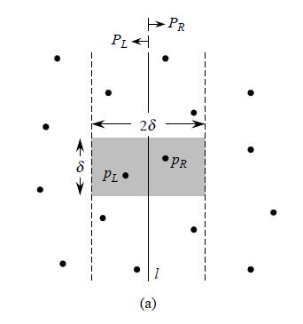
(picture: the points around line l. source: CLRS P1042)

Step 1: Sort the points by X-axis value, then divide points based on the middle points. Q[0, end] divided into Q1[0,m] and Q2[m+1,end].

Step 2: compute the minimum distance $\delta$ of points in Q1 and Q2.

Step 3: Find the points with a distance to line $x = Q[m][0]$ smaller than $\delta$ . For each point $P_L1(x1,y1)$ in $P_L$ . on the left of the line, compute the distance between p and one points in the area of $\{y|y1 + \delta > y \}$ . We only need to compute at most 6 points

Step 4: return the minimum distance of point pair.

The difficult part of Closest pair of points is finding the closest points around line l. It was proof by Preparata and Shamos that given a point $P_L1(x1,y1)$ in $P_L$ . There are at most 6 points in the area: $\{x,y| l < x < l + \delta, y1 - \delta < y < y1+ \delta\}$ . Therefore for each points in $P_L$ , we only need to check at most 6 points, that significantly reduced the time complexity.

#include <vector>
#include <algorithm>
#include <iostream>
#include <cmath>

using namespace std;
struct Point
{
	double x;
	double y;
};
inline double dis(const Point& p1, const Point& p2)
{
	return sqrt(pow(p1.x - p2.x, 2) + pow(p1.y - p2.y, 2));
}
struct min_pair
{
	Point p1;
	Point p2;
	double min_dis = dis(p1,p2);
};
bool cmpx(const Point& p1, const Point& p2)
{
	return p1.x < p2.x ;
}
bool cmpy(const Point& p1, const Point& p2)
{
	return p1.y < p2.y;
}
bool dis_cmp(const min_pair& m1, const min_pair& m2)
{
	return m1.min_dis < m2.min_dis;
}
vector<Point> points;
min_pair find_closest(int l, int r) {
	int m = (l + r) / 2;
	int len = r - l + 1;
	if (len == 2) {
		return { points[l],points[r] };
	}
	else if (len == 3)
	{
		min_pair ps1,ps2,ps3,ret;
		ps1 = { points[l],points[l + 1] };
		ps2 = { points[l],points[r] };
		ps3 = { points[l + 1],points[r] };
		ret = min(ps1, ps2, dis_cmp);
		ret = min(ps3, ret, dis_cmp);
		return ret;
	}
	else
	{
		min_pair m1, m2, m3;
		m1 = find_closest(l, m);
		m2 = find_closest(m, r);
		m3 = min(m1, m2, dis_cmp);
		//find points in  m +- theta
		vector<Point> left, right;
		for (int i = l; i < r; ++i)
		{
			if (points[i].x - points[m].x <= 0 && points[i].x - points[m].x > -m3.min_dis)
				left.push_back(points[i]);
			else if (points[i].x - points[m].x > 0 && points[i].x - points[m].x < m3.min_dis)
				right.push_back(points[i]);
		}
		sort(right.begin(), right.end(),cmpy);
		for (Point& p : left)
		{
			int i = 0;
			for (i = 0; i < right.size() && p.y < right[i].y - m3.min_dis; ++i);
			for (int j = 0; j < 7 && i + j < right.size(); ++j) 
			{
				if (dis(left[i], right[j + i]) < m3.min_dis)
				{
					m3 = { left[i],right[j + i],dis(left[i], right[j + i]) };
				}
			}
		}
		return m3;
	}
}
int main() {
	double d1,d2;
	while (cin >> d1 >>d2)
	{
		points.push_back({ d1,d2 });
	}
	int r = points.size()-1;
	min_pair final_m;
	sort(points.begin(), points.end(), cmpx);
	cout << "the point set is : ";
	for (auto& p : points) {
		cout << p.x << ", " << p.y << "; ";
	}
	final_m = find_closest(0, r);
	cout << "\nminimum distance is ：  " << final_m.min_dis;
	cout << "\n Closest pair of points are ： "<<	final_m.p1.x << ","<< final_m.p1.y;
	cout << " and "<< final_m.p2.x <<","<< final_m.p2.y << endl;
	return 0;
}

Hanoi

Hanoi is not that difficult, but interesting. As the last one example, some conclusion of this topic will be made in this part.

You might find the solution for Hanoi towel through 2 ways.

First, list the result for $n = 1,2,3, 4,5$ . And they might find $result = 1, 3, 7, 15, 31$ . It make sense to guess that the $result = 2^n -1$ . Second is to proof it, if we consider the top n-1 level of towel as a whole. We only need 3 steps to finish the game: 1. Move the top n-1 level. 2. Move the last level. 3. Move the top n-1 level. So the $result\ of\ n\ level = 2 * (result\ of\ n-1\ level) + 1$ . Use induction can proof $result = 2^n - 1$

Therefore, a key to find a divide and conquer algorithm for solving some question is observing the features of result, and try to figure out the relationship between problem and sub problem. Given that, it is quite simple to solve all kinds of Hanoi problem. For example, assume you are moving a 14 level Hanoi towel. However, owning to the dinner, you have to stopped at some point. When you come back, how to know what is the next step, and how many steps you left in order to finish the game?

# Original Hanoi towel
def original_hanoi(n,A,B,C):
    if n > 0:
        original_hanoi(n-1,A,C,B)
        [A,B,C][2].insert(0,[A,B,C][0].pop(0))   
        print([A,B,C])
        original_hanoi(n-1,B,A,C)

Divide-and-conquer|分治算法

# Merge Sort

# QuickSort

# Closest Pair of Points

# Hanoi

Merge Sort

QuickSort

Closest Pair of Points

Hanoi