Basic DL Notes

Basic Deep Learning math for Coursera Course Deep Learning by Andrew Ng, Kian Katanforoosh and Younes Bensouda Mourri.

Please expect some loading time due to math formula.

Basic NN

Matrix size: m training examples, n_x features. Matrix.shape = (n_x,m)

Activation function:

$$\begin{array}{l} a=\tanh (z) =\frac{e^{z}-e^{-z}}{e^{z}+e^{-z}} \end{array}$$

$$\tanh' (z) =1-(\tanh(z))^2$$

Relu: $A = RELU(Z) = max(0, Z)$

Logistic regression with sigmoid: $\hat y = \sigma (w^Tx + b)$ ,when $x_0 = 1, \hat y = \sigma(\theta^Tx)$

Logistic Regression loss function: $L(\hat{y}, y)=-(y \log \hat{y}+(1-y) \log (1-\hat{y}))$

Logistic cost function:

$$J(w,b) = 1/m \sum_{i=1} ^m L(\hat {y^i},y^i)\\= -\frac{1}{m} \sum\limits_{i = 1}^{m} (y^{(i)}\log\left(a^{[L] (i)}\right) + (1-y^{(i)})\log\left(1- a^{[L](i)}\right))$$

Gradient decent: $w -= \alpha \frac {d J(w)}{ d (w)}$

partial derivative: Do check the relationship of $x_1$ and other parameters.

$$\begin{aligned} &z=f(x_1, x_2)\\ &\frac{\partial z}{\partial x_1 }=f_{1}^{\prime} \cdot \frac{\partial x_1}{\partial x_1}+f_{2}^{\prime} \cdot \frac{\partial x_2}{\partial x_1}=f_{1}^{\prime}+ f_{2}^{\prime}\frac{\partial x_2}{\partial x_1} \end{aligned}$$

Chain rule: $\frac {dJ}{dv} \frac {dV}{da} = \frac {dJ}{da}$

Logistic Derivative (sigmoid):

$$a = \sigma (z)\\ \frac {dL(a,y)}{da} = -\frac ya + \frac {1-y}{1-a}\\ \frac {dL(a,y)}{dz} =a-y\\ \frac {dL(a,y)}{dw_i} = x_i\frac {dL(a,y)}{dz}(when\ i=0,w_i\ is\ b)\\ \frac{\partial J(w, b)}{\partial w_{1}}=\frac{1}{m} \sum_{i=1}^{m} \frac{\partial}{\partial w_{i}} L\left(a^{(i)}, y^{(i)} \right)$$

Vectorization: $z = w^T x$

Softmax function:

$$\text{for } x \in \mathbb{R}^{1\times n} \text{, } softmax(x) = \\softmax(\begin{bmatrix} x_1 && x_2 && ... && x_n \end{bmatrix}) \\= \begin{bmatrix} \frac{e^{x_1}}{\sum_{j}e^{x_j}} && \frac{e^{x_2}}{\sum_{j}e^{x_j}} && ... && \frac{e^{x_n}}{\sum_{j}e^{x_j}} \end{bmatrix}$$

$$softmax(x) = \\softmax\begin{bmatrix} x_{11} & x_{12} & x_{13} & \dots & x_{1n} \\ x_{21} & x_{22} & x_{23} & \dots & x_{2n} \\ \vdots & \vdots & \vdots & \ddots & \vdots \\ x_{m1} & x_{m2} & x_{m3} & \dots & x_{mn} \end{bmatrix} \\ = \begin{bmatrix} \frac{e^{x_{11}}}{\sum_{j}e^{x_{1j}}} & \frac{e^{x_{12}}}{\sum_{j}e^{x_{1j}}} & \frac{e^{x_{13}}}{\sum_{j}e^{x_{1j}}} & \dots & \frac{e^{x_{1n}}}{\sum_{j}e^{x_{1j}}} \\ \frac{e^{x_{21}}}{\sum_{j}e^{x_{2j}}} & \frac{e^{x_{22}}}{\sum_{j}e^{x_{2j}}} & \frac{e^{x_{23}}}{\sum_{j}e^{x_{2j}}} & \dots & \frac{e^{x_{2n}}}{\sum_{j}e^{x_{2j}}} \\ \vdots & \vdots & \vdots & \ddots & \vdots \\ \frac{e^{x_{m1}}}{\sum_{j}e^{x_{mj}}} & \frac{e^{x_{m2}}}{\sum_{j}e^{x_{mj}}} & \frac{e^{x_{m3}}}{\sum_{j}e^{x_{mj}}} & \dots & \frac{e^{x_{mn}}}{\sum_{j}e^{x_{mj}}} \end{bmatrix} \\= \begin{pmatrix} softmax\text{(first row of x)} \\ softmax\text{(second row of x)} \\ ... \\ softmax\text{(last row of x)} \\ \end{pmatrix}$$

Bias & Variance & human level performance:

• it is important to clear Bayes error

%	high variance	high bias	bias + variance
Dev set error	11	16	30
Train set error	1	15	15
optimal (Bayes) error	0%	0	0

L2 regularization:

$J_{regularized} = \small \underbrace{-\frac{1}{m} \sum\limits_{i = 1}^{m} \large{(}\small y^{(i)}\log\left(a^{[L](i)}\right) + (1-y^{(i)})\log\left(1- a^{[L](i)}\right) \large{)} }_\text{cross-entropy cost} + \underbrace{\frac{1}{m} \frac{\lambda}{2} \sum\limits_l\sum\limits_k\sum\limits_j W_{k,j}^{[l]2} }_\text{L2 regularization cost}$

Dropout: randomly close some nodes

D1 = np.random.rand(A1.shape[0],A1.shape[1])
D1 = D1 < keep_prob
A1 = A1*D1
A1 = A1/keep_prob

He initialization: after np.random.randn(..,..), multiply the initialized random value by$\sqrt{\frac{2}{\text{dimension of the previous layer}}}$

Mini-batch gradient descent:

• If mini-batch size == 1, noise up, stochastic Gradient Descent. If mini-batch == m, time cost up, batch gradient descent.
• small training set (m<2000) use batch gradient.
• mini-batch size recommend to set as $2^n$ to fit GPU, CPU memory.

Momentum: Momentum takes into account the past gradients to smooth out the update.

$$\begin{cases} v_{dW^{[l]}} = \beta v_{dW^{[l]}} + (1 - \beta) dW^{[l]} \\ W^{[l]} = W^{[l]} - \alpha v_{dW^{[l]}} \end{cases}$$

$$\begin{cases} v_{db^{[l]}} = \beta v_{db^{[l]}} + (1 - \beta) db^{[l]} \\ b^{[l]} = b^{[l]} - \alpha v_{db^{[l]}} \end{cases}$$

where L is the number of layers, 𝛽 is the momentum and 𝛼 is the learning rate. Common values for 𝛽 range from 0.8 to 0.999

RMSprop:

$$s_{dW^{[l]}} = \beta_2 s_{dW^{[l]}} + (1 - \beta_2) (\frac{\partial \mathcal{J} }{\partial W^{[l]} })^2 \\ W^{[l]} = W^{[l]} - \alpha\frac {dW^ {[l]}}{\sqrt {S_{dW^{[l]}}+\epsilon}}$$

Adam:

$$\begin{cases} v_{dW^{[l]}} = \beta_1 v_{dW^{[l]}} + (1 - \beta_1) \frac{\partial \mathcal{J} }{ \partial W^{[l]} } \\ v^{corrected}_{dW^{[l]}} = \frac{v_{dW^{[l]}}}{1 - (\beta_1)^t} \\ s_{dW^{[l]}} = \beta_2 s_{dW^{[l]}} + (1 - \beta_2) (\frac{\partial \mathcal{J} }{\partial W^{[l]} })^2 \\ s^{corrected}_{dW^{[l]}} = \frac{s_{dW^{[l]}}}{1 - (\beta_2)^t} \\ W^{[l]} = W^{[l]} - \alpha \frac{v^{corrected}_{dW^{[l]}}}{\sqrt{s^{corrected}_{dW^{[l]}}} + \varepsilon} \end{cases}$$

where:

• t counts the number of steps taken of Adam
• $\beta_1$ and $\beta_2$ are hyperparameters that control the two exponentially weighted averages. $\beta_1$ around 0.9, $\beta_2$ around 0.999
• $\varepsilon$ is a very small number ($10^{-8}$) to avoid dividing by zero.

Gradient Checking:

$$\frac{\partial J}{\partial \theta} = \lim_{\varepsilon \to 0} \frac{J(\theta + \varepsilon) - J(\theta - \varepsilon)}{2 \varepsilon}$$

Learning rate decay:

Learning rate $\alpha = \frac {\alpha_0}{1+decay\_rate\ *\ epoch\_num}$ or $\alpha = 0.95 ^{epoch\ num} * \alpha_0$ or $\alpha = \frac k{\sqrt {epoch\ num}} * \alpha_0$ or manual decay

Tuning process: 1. $\alpha$ 2. $\beta, \beta_1, \beta_2$, #layers, mini batch size 3. ​# layers, learning rate decay. Do not use grid, choose random number

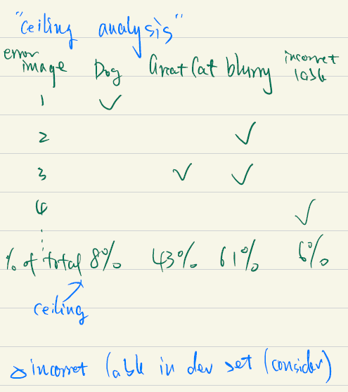
Error Analysis:

• Consider Train, Test different or Train, Dev different.

相关图片

Artificial Data Synthesis: if just synthesize a small subset, you will overfit to the synthesize subset.

相关图片

Transfer Learning: Task A B have same input, low level feature from A could help for learning B.

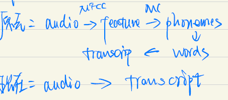
End-to-end learning: e.g. speech recognition. Need large amount of data. Let data speak, less hand-designed needed.

相关图片

Computer Visualization

CNN

padding:

• same convolution:

$$\text {input size = pad and output size}\\ n + 2p - f + 1 = n\\ p = \frac {f-1}2\\ f\ usually\ odd$$

• valid convolution: no padding. input size $n * n$, filter size $f*f$, output size $n-f+1$

stride convolutions: for stride = 2, output size is

$$\lfloor\frac{n+2 p-f}{s}+1 \rfloor * \lfloor\frac{n+2 p-f}{s}+1 \rfloor$$

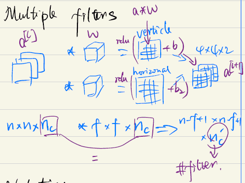
multiple filters:

相关图片

codes for understand process only

def conv_forward(A_prev, W, b, stride, pad):
    (m, n_H_prev, n_W_prev, n_C_prev) = A_prev.shape
    (f, f, n_C_prev, n_C) = W.shape   
	# output dimension
    n_H = int((n_H_prev-f+2* pad)/stride)+1
    n_W = int((n_W_prev-f+2* pad)/stride)+1
    
    Z = np.zeros((m,n_H,n_W,n_C))
    A_prev_pad = zero_pad(A_prev, pad)
    
    for i in range(m): # m example
        a_prev_pad = A_prev_pad[i,:,:,:] 
        for h in range(n_H):
            vert_start = h * stride
            vert_end = vert_start + f
            for w in range(n_W): 
                horiz_start = w * stride
                horiz_end = horiz_start + f
                for c in range(n_C):  # c: number of channels(filters) in each layer
                    a_slice_prev = a_prev_pad[vert_start:vert_end,horiz_start:horiz_end,:]
                    weights = W[:,:,:,c]
                    biases = b[:,:,:,c]
                    Z[i, h, w, c] = conv_single_step(a_slice_prev, weights, biases)
    cache = (A_prev, W, b, hparameters)
    
    return Z, cache

Pooling Layer: Max pooling, Average pooling

Convolutional NN backpropagation:

$dA += \sum _{h=0} ^{n_H} \sum_{w=0} ^{n_W} W_c \times dZ_{hw}$

$dW_c += \sum _{h=0} ^{n_H} \sum_{w=0} ^ {n_W} a_{slice} \times dZ_{hw}$

$db = \sum_h \sum_w dZ_{hw}$

mask for max pooling backward pass, average for average pooling backward pass

Model Examples Summary

Notation:

• filter: [filter size, stride]
• A: (Height, Width, Channel)

LeNet-5 (activation: sigmoid or tanh)

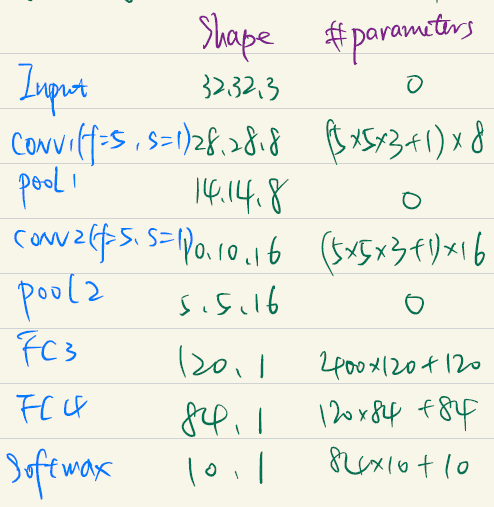
$(32,32,3) \rightarrow [5,1]\rightarrow (28,28,6)\rightarrow maxpool[2,2]$

$\rightarrow (14,14,6) \rightarrow [5,1] \rightarrow(10,10,10)\rightarrow maxpool[2,2]$

$\rightarrow (5,5,16) \rightarrow flatten \rightarrow 400\rightarrow FC3:120$

$\rightarrow FC4:84 \rightarrow 10,softmax \rightarrow output$

相关图片

AlexNet (Relu)

$(227,227,3) \rightarrow [11,4]\rightarrow (55,55,96)\rightarrow maxpool[3,2]$

$\rightarrow (27,27,96) \rightarrow same[5,1] \rightarrow(27,27,256)\rightarrow maxpool[3,2]$

$\rightarrow (13,13,256) \rightarrow same[3,1] \rightarrow (13,13,384) \rightarrow same[3,1]$

$\rightarrow (13,13,384) \rightarrow same[3,1]\rightarrow(13,13,256) \rightarrow maxpool[3,2]$

$\rightarrow (6,6,256) \rightarrow flatten \rightarrow 9216 \rightarrow FC:4096$

$\rightarrow FC:4096\rightarrow softmax$

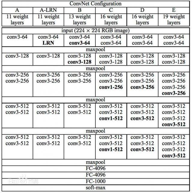
VGG-16 (source code here)

c2fdfc039245d6888f2a8c35134ecc18d31b248d

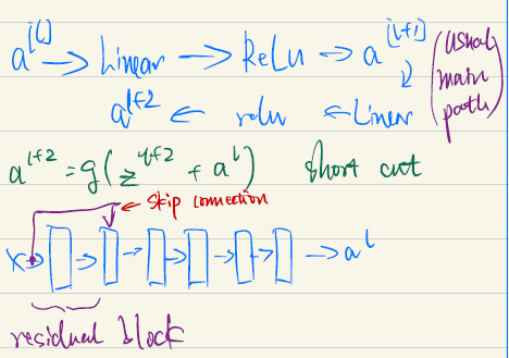
Residual Network (ResNets)

• ResNets not hurt NN, if lucky can help.

source code

相关图片

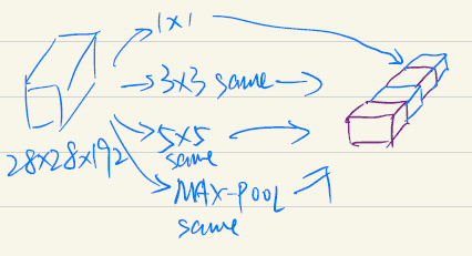
Inception net keras source code

相关图片

Data argumentation: 1. mirroring 2. random cropping 3. rotation shearing, local wraping 4. color shifting

YOLO

bounding box: $b_x,b_y,b_h,b_w$ : middle point,height, width

Anchor boxes : same box overlap objects

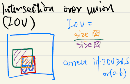
Intersection over union

相关图片

Non-max suppression

• discard all picture with low score (e.g. <0.6)
• select only one box (e.g. with max score) when several boxes overlap with each other and detect the same object.

Face recognition

Make sure Anchor image is closer to Positive image then to Negative image by at least a margin $\alpha$.

$\mid \mid f(A^{(i)}) - f(P^{(i)}) \mid \mid_2^2 + \alpha < \mid \mid f(A^{(i)}) - f(N^{(i)}) \mid \mid_2^2$

minimize the triplet cost:

$\mathcal{J} = \sum^{m}_{i=1} \large[ \small \underbrace{\mid \mid f(A^{(i)}) - f(P^{(i)}) \mid \mid_2^2}_\text{(1)} - \underbrace{\mid \mid f(A^{(i)}) - f(N^{(i)}) \mid \mid_2^2}_\text{(2)} + \alpha \large ] \small_+$

Neural Style transfer

Notation: $a^{(C)}$ : the hidden layer activations in the layer after running content image C in network.

Notation: $a^{(G)}$ : the hidden layer activations in the layer after running generated image G in network.

$J_{content}(C,G) = \frac{1}{4 \times n_H \times n_W \times n_C}\sum _{ \text{all entries}} (a^{(C)} - a^{(G)})^2$

• The content cost takes a hidden layer activation of the neural network, and measures how different 𝑎(𝐶) and 𝑎(𝐺) are.
• When we minimize the content cost later, this will help make sure 𝐺 has similar content as 𝐶.

Gram matrix

Notation: $\mathbf{G}_{gram} = \mathbf{A}_{unrolled} \mathbf{A}_{unrolled}^T$

Notation: $G_{(gram)i,j}$ : correlation of activations of filter i and j

Notation: $G_{(gram),i,i}$ : prevalence of patterns or textures

• The diagonal elements $G_{(gram)ii}$ measure how "active" a filter $i$ is.
• For example, suppose filter $i$ is detecting vertical textures in the image. Then $G_{(gram)ii}$ measures how common vertical textures are in the image as a whole.
• If $G_{(gram)ii}$ is large, this means that the image has a lot of vertical texture.

Style cost: $J_{style}^{[l]}(S,G) = \frac{1}{4 \times {n_C}^2 \times (n_H \times n_W)^2} \sum _{i=1}^{n_C}\sum_{j=1}^{n_C}(G^{(S)}_{(gram)i,j} - G^{(G)}_{(gram)i,j})^2$

Combine style cost for different layers: $J_{style}(S,G) = \sum_{l} \lambda^{[l]} J^{[l]}_{style}(S,G)$

HINTS:

• The style of an image can be represented using the Gram matrix of a hidden layer's activations.
• We get even better results by combining this representation from multiple different layers.
• This is in contrast to the content representation, where usually using just a single hidden layer is sufficient.
• Minimizing the style cost will cause the image 𝐺G to follow the style of the image 𝑆S.

Total cost to optimize: $J(G) = \alpha J_{content}(C,G) + \beta J_{style}(S,G)$

• The total cost is a linear combination of the content cost $J_{content}(C,G)$ and the style cost $J_{style}(S,G)$.
• $\alpha$ and $\beta$ are hyperparameters that control the relative weighting between content and style.

RNN

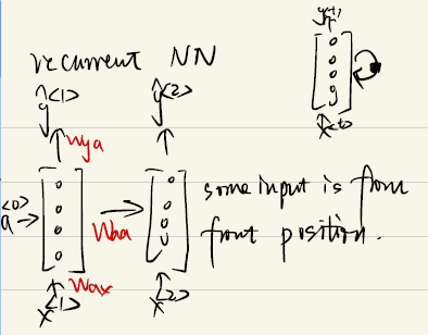
Basic RNN

相关图片

Forward Propagation

$$a^{\langle t \rangle} = \tanh(W_{aa} a^{\langle t-1 \rangle} + W_{ax} x^{\langle t \rangle} + b_a)\\\hat{y}^{\langle t \rangle} = softmax(W_{ya} a^{\langle t \rangle} + b_y)$$

Backpropagation

$$\displaystyle {dW_{ax}} = da_{next} * ( 1-\tanh^2(W_{ax}x^{\langle t \rangle}+W_{aa} a^{\langle t-1 \rangle} + b_{a}) ) x^{\langle t \rangle T}\\ \displaystyle dW_{aa} = da_{next} * (( 1-\tanh^2(W_{ax}x^{\langle t \rangle}+W_{aa} a^{\langle t-1 \rangle} + b_{a}) ) a^{\langle t-1 \rangle T}\\ \displaystyle db_a = da_{next} * \sum_{batch}( 1-\tanh^2(W_{ax}x^{\langle t \rangle}+W_{aa} a^{\langle t-1 \rangle} + b_{a}) )\\ \displaystyle dx^{\langle t \rangle} = da_{next} * { W_{ax}}^T ( 1-\tanh^2(W_{ax}x^{\langle t \rangle}+W_{aa} a^{\langle t-1 \rangle} + b_{a}) )\\ \displaystyle da_{prev} = da_{next} * { W_{aa}}^T ( 1-\tanh^2(W_{ax}x^{\langle t \rangle}+W_{aa} a^{\langle t-1 \rangle} + b_{a}) )$$

Gate Recurrent Unit

Forward Propagation

$$\mathbf{\tilde{c}}^{\langle t \rangle} = \tanh\left( \mathbf{W}_{c} [\mathbf{\Gamma}_r^{\langle t \rangle} * \tanh(\mathbf{c}^{\langle t-1 \rangle}), \mathbf{x}^{\langle t \rangle}] + \mathbf{b}_{c} \right)\\ \mathbf{\Gamma}_u^{\langle t \rangle} = \sigma(\mathbf{W}_u[\mathbf{c}^{\langle t-1 \rangle}, \mathbf{x}^{\langle t \rangle}] + \mathbf{b}_u) \\ \mathbf{\Gamma}_r^{\langle t \rangle} = \sigma(\mathbf{W}_r[\mathbf{c}^{\langle t-1 \rangle}, \mathbf{x}^{\langle t \rangle}] + \mathbf{b}_c) \\ \mathbf{c}^{\langle t \rangle} = \mathbf{\Gamma}_u^{\langle t \rangle} * \mathbf{\tilde{c}}^{\langle t \rangle} + (1-\mathbf{\Gamma}_u^{\langle t \rangle})*\mathbf{c}^{\langle t-1 \rangle} \\ \mathbf{a}^{\langle t \rangle} = \mathbf{c}^{\langle t \rangle}$$

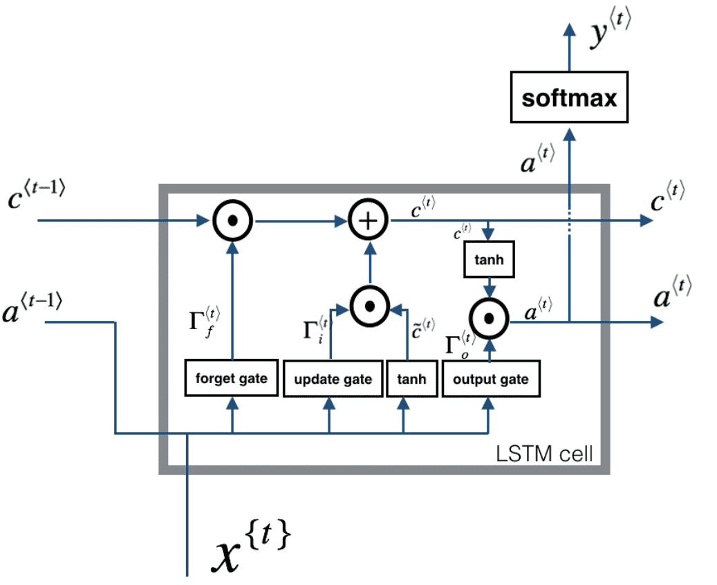
LSTM

LSTM cell

相关图片

Forward Propagation

v2-1bc8771964da03fa090223d8604b6536_r

$$\mathbf{\tilde{c}}^{\langle t \rangle} = \tanh\left( \mathbf{W}_{c} [\mathbf{a}^{\langle t - 1 \rangle}, \mathbf{x}^{\langle t \rangle}] + \mathbf{b}_{c} \right)\\ \mathbf{\Gamma}_i^{\langle t \rangle} = \sigma(\mathbf{W}_i[a^{\langle t-1 \rangle}, \mathbf{x}^{\langle t \rangle}] + \mathbf{b}_i)\\ \mathbf{\Gamma}_f^{\langle t \rangle} = \sigma(\mathbf{W}_f[\mathbf{a}^{\langle t-1 \rangle}, \mathbf{x}^{\langle t \rangle}] + \mathbf{b}_f)\\ \mathbf{c}^{\langle t \rangle} = \mathbf{\Gamma}_f^{\langle t \rangle}* \mathbf{c}^{\langle t-1 \rangle} + \mathbf{\Gamma}_{i}^{\langle t \rangle} *\mathbf{\tilde{c}}^{\langle t \rangle}\\ \Gamma ^{\langle t\rangle }_o=\sigma (\mathbf{W}_o[𝐚^{\langle t-1\rangle },x^{\langle t\rangle }]+b_o)\\ 𝐚^{\langle t\rangle }=\Gamma ^{\langle t\rangle }_o∗tanh(𝐜^{\langle t\rangle })\\ 𝐲^{\langle t\rangle }_{𝑝𝑟𝑒𝑑}=softmax(\mathbf{W}_𝑦𝐚^{\langle t\rangle }+b_𝑦)$$

concatenate hidden state and input into single matrix: $concat = \begin{bmatrix} a^{\langle t-1 \rangle} \\ x^{\langle t \rangle} \end{bmatrix}$

Backpropagation

Notation: $\Gamma_u^{\langle t \rangle}$ is same as $\Gamma_i^{\langle t \rangle}$ in previous discussion.

$$\displaystyle \frac{\partial \tanh(x)} {\partial x} = 1 - \tanh^2(x) \\ \displaystyle \frac{\partial \sigma(x)} {\partial x} = (1-\sigma(x)) * \sigma (x)$$

in the following, $\gamma_o^{\langle t \rangle} = \mathbf{W}_o[𝐚^{\langle t-1\rangle },x^{\langle t\rangle }]+b_o$. Same for $\gamma_u^{\langle t \rangle}, \gamma_f^{\langle t \rangle} $

$$d\gamma_o^{\langle t \rangle} = da_{next}*\tanh(c_{next}) * \Gamma_o^{\langle t \rangle}*\left(1-\Gamma_o^{\langle t \rangle}\right)\\ dp\widetilde{c}^{\langle t \rangle} = \left(dc_{next}*\Gamma_u^{\langle t \rangle}+ \Gamma_o^{\langle t \rangle}* (1-\tanh^2(c_{next})) * \Gamma_u^{\langle t \rangle} * da_{next} \right) * \left(1-\left(\widetilde c^{\langle t \rangle}\right)^2\right)\\ d\gamma_u^{\langle t \rangle} = \left(dc_{next}*\widetilde{c}^{\langle t \rangle} + \Gamma_o^{\langle t \rangle}* (1-\tanh^2(c_{next})) * \widetilde{c}^{\langle t \rangle} * da_{next}\right)*\Gamma_u^{\langle t \rangle}*\left(1-\Gamma_u^{\langle t \rangle}\right)\\ d\gamma_f^{\langle t \rangle} = \left(dc_{next}* c_{prev} + \Gamma_o^{\langle t \rangle} * (1-\tanh^2(c_{next})) * c_{prev} * da_{next}\right)*\Gamma_f^{\langle t \rangle}*\left(1-\Gamma_f^{\langle t \rangle}\right)\\$$

$$dW_k = d\gamma_k^{\langle t \rangle} \begin{bmatrix} a_{prev} \\ x_t\end{bmatrix}^T \text{, for k = o, u, f}\\ dW_c = dp\widetilde c^{\langle t \rangle} \begin{bmatrix} a_{prev} \\ x_t\end{bmatrix}^T\\ \displaystyle db_k = \sum_{batch}d\gamma_k^{\langle t \rangle} \text{ , for k = o, u, f, c}$$

$$da_{prev} = W_f^T d\gamma_f^{\langle t \rangle} + W_u^T d\gamma_u^{\langle t \rangle}+ W_c^T dp\widetilde c^{\langle t \rangle} + W_o^T d\gamma_o^{\langle t \rangle}\\ dc_{prev} = dc_{next}*\Gamma_f^{\langle t \rangle} + \Gamma_o^{\langle t \rangle} * (1- \tanh^2(c_{next}))*\Gamma_f^{\langle t \rangle}*da_{next}\\ dx^{\langle t \rangle} = W_f^T d\gamma_f^{\langle t \rangle} + W_u^T d\gamma_u^{\langle t \rangle}+ W_c^T dp\widetilde c^{\langle t \rangle} + W_o^T d\gamma_o^{\langle t \rangle}$$

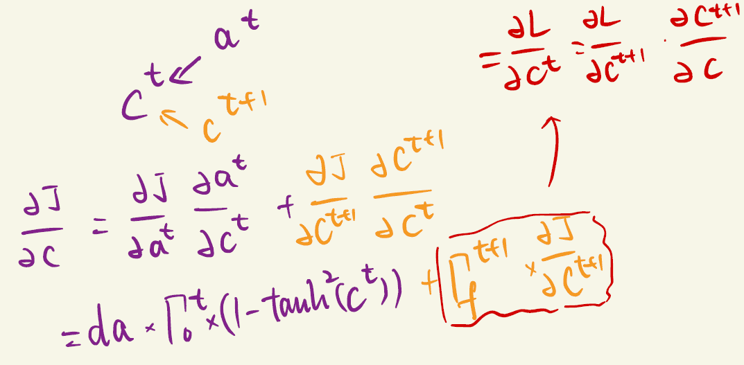
Parameter source hints for partial derivative: $\Gamma ^{\langle t\rangle }_o$ : $\mathbf{a}^{\langle t \rangle}$ , $\Gamma ^{\langle t\rangle }_u$ and $\Gamma ^{\langle t\rangle }_f$: $\mathbf{c}^{\langle t \rangle}$, $\mathbf{\tilde{c}}^{\langle t \rangle}$ : $\mathbf{c}^{\langle t \rangle}$ , $\mathbf{c}^{\langle t \rangle}$: $\mathbf{c}^{\langle t+1 \rangle} , \mathbf{a}^{\langle t \rangle}$ , $\frac{\partial J} {\partial c^{<t>}}$

相关图片

NLP

Word2Vec

Cosine similarity: $\text{CosineSimilarity(u, v)} = \frac {u \cdot v} {||u||_2 ||v||_2} = cos(\theta)$

Debiasing word vectors:

Neutralize bias for non-gender specific words

$$e^{bias\_component} = \frac{e \cdot g}{||g||_2^2} * g\\ e^{debiased} = e - e^{bias\_component}$$

Equalization algorithm for gender-specific words

$$\mu = \frac{e_{w1} + e_{w2}}{2} \\ \mu_{B} = \frac {\mu \cdot \text{bias axis}}{||\text{bias axis}||_2^2} *\text{bias axis}\\ \mu_{\perp} = \mu - \mu_{B} \\ e_{w1B} = \frac {e_{w1} \cdot \text{bias axis}}{||\text{bias axis}||_2^2} *\text{bias axis}\\ e_{w2B} = \frac {e_{w2} \cdot \text{bias axis}}{||\text{bias axis}||_2^2} *\text{bias axis}\\ e_{w1B}^{corrected} = \sqrt{ |{1 - ||\mu_{\perp} ||^2_2} |} * \frac{e_{\text{w1B}} - \mu_B} {||(e_{w1} - \mu_{\perp}) - \mu_B||} \\ e_{w2B}^{corrected} = \sqrt{ |{1 - ||\mu_{\perp} ||^2_2} |} * \frac{e_{\text{w2B}} - \mu_B} {||(e_{w2} - \mu_{\perp}) - \mu_B||} \\ e_1 = e_{w1B}^{corrected} + \mu_{\perp} \\ e_2 = e_{w2B}^{corrected} + \mu_{\perp}$$

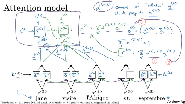
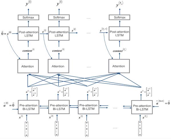
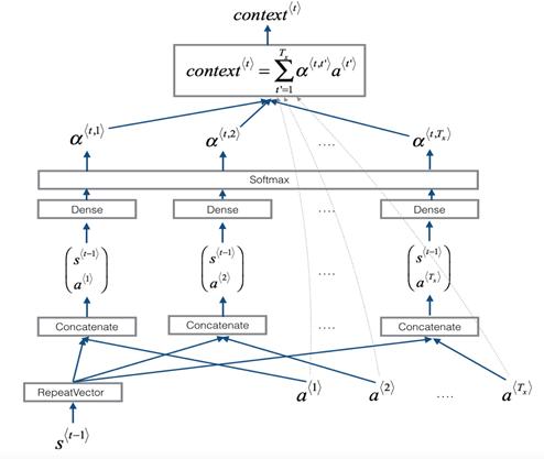
Attention model

$$\alpha^{<t, t^{\prime}>}=\frac{\exp \left(e^{<t, t^{\prime}>}\right)}{\sum_{t^{\prime}=1}^{T x} \exp \left(e^{<t, t^{\prime}>}\right)}$$

13931179-a6577be388e416f6

相关图片

相关图片