NLP BASELINE

Summary for application and theory for NLP baseline model. Sample code please referred to My github.

Even we do not use them today, however, learning the baseline models are important for understanding on how to encode and decode a language, which is the priority of NLP.

Logistic Regression

STEPS

1. Preprocessing

Stop words and punctuation

Stemming and lowercasing

Tokenize sentences

2. Feature Extraction with frequency

相关图片

相关图片

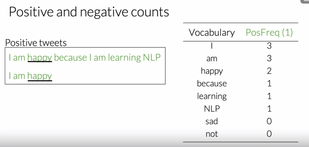
the sum is for unique words, do duplicate.

3. Train Logistic model for sentiment analysis based on the features

Naive Bayes

Steps

1. Get or annotate a dataset with positive and negative tweets

2. Preprocess tweet

3. Get Word count

相关图片

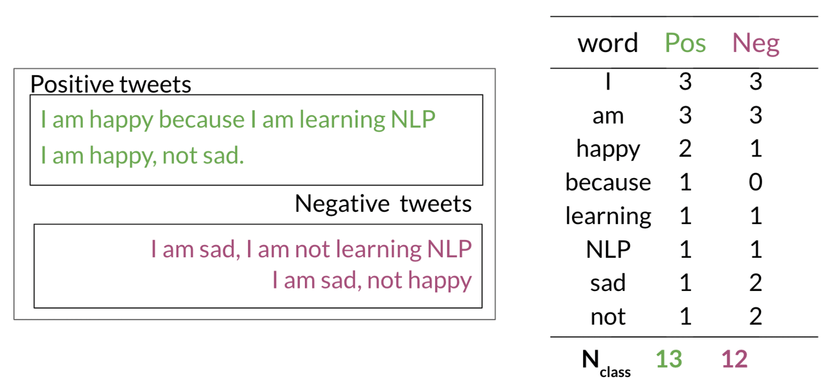
4. Get Frequency tables

相关图片

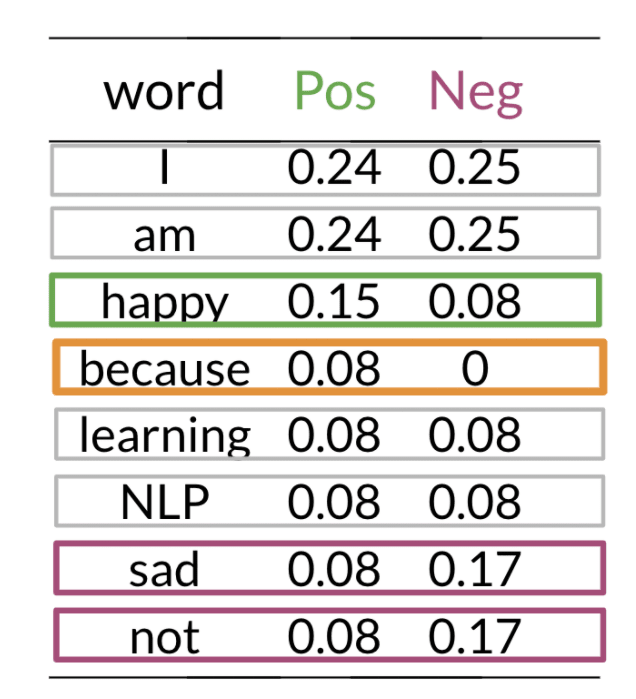
5. Apply Laplacian Smoothing to avoid P = 0

$$P\left(\mathrm{w}_{\mathrm{i}} \mid \text { class }\right)=\frac{\text { freq }\left(\mathrm{w}_{\mathrm{i}}, \text { class }\right)+1}{\mathrm{N}_{\text {class }}+\mathrm{V}}$$

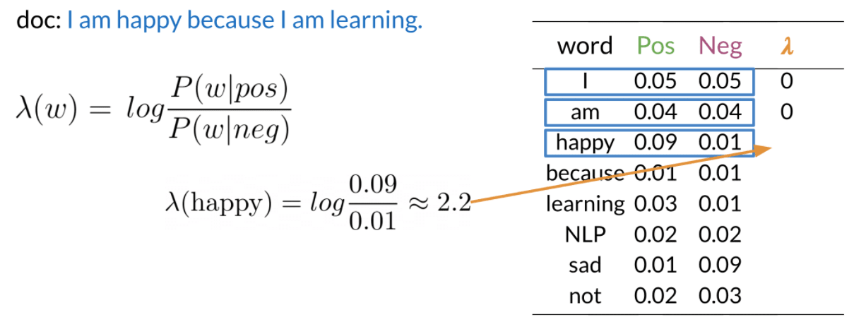
6. Compute Log likelihood - lambda

$$\lambda(w)=\log \frac{P(\mathrm{w} \mid \mathrm{pos})}{P(\mathrm{w} \mid \mathrm{neg})}$$

相关图片

7. Compute log prior

The $D_{pos}$ and $D_{neg}$ correspond to number of positive and negative tweet

$$\log(\frac {D(pos)}{D(neg)})$$

8. Made prediction

when prediction, we assume that the unknown word do not provide any information.

相关图片

$$\log P(pos|w_1,w_2,..,w_n) =\log \frac { P(w_1,w_2,..,w_n|pos) \times P(pos)}{P(w_1,w_2,..w_n)}\\ \log P(pos|w_1,..w_n)- \log P(neg|w_1,..,w_n) = \log \frac{D_{pos}}{D_{neg}} + \sum_i\lambda(w_i)$$

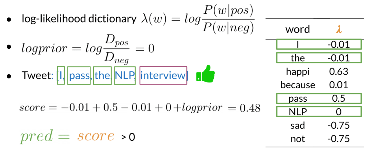
Assumptions

Independence assumption

It is always cold and snowy in __.

Naive Bayes assumes independence throughout. Furthermore, if you were to fill in the sentence on the right, this naive model will assign equal weight to the words "spring, summer, fall, winter".

Relative frequencies in corpus

In real word, there are much more positive tweets than negative. And the data could be much noisier.

Consideration

To speed up the prediction and training time, we might filter those word with neutral sentiment, that is filter based on the POS/NEG ratio.

Error Analysis

Removing punctuation and stop words

• I love learning 😦
• removing not making sentence being positive

Word order

• I am happy because I did not go

Adversarial attacks

• sarcasm, irony and Euphemisms

Example:

Tweet:

This is a ridiculously powerful movie. The plot was gripping and cried right through until the ending! processed tweet:

[ridicul, power, movi, plot, grip, cry, end] looks not good.

Vector Space Models

Instead of using The above 2 base model, a advance way is encoding words as vector. Encoding a text as a vector, Vector spaces are fundamental in many applications in NLP.

You can encode different relationship to get different performance.

• word by word (such as n-gram) and word by doc (the center word changed to a doc)
  • The idea is encode word or doc using word frequency.
  • if possible, you can try encode word using doc frequency, topic frequency etc.

Word Embedding (1) - PCA/SVD

A unsupervised-learning approach for getting word Embedding

STEPS:

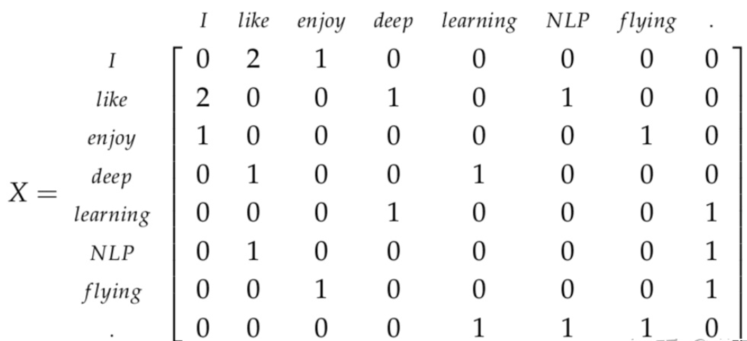
1. Compute Window based Co-occurrence Matrix

Given following text, and window size being 3.

• I enjoy flying。

• I like NLP。

• I like deep learning。

Get Co-occurrence matrix:

相关图片

2. Apply SVD and select the first K columns

One of the method is usenp.linalg.SVD. the first k columns of matrix U is the word vectors (word embeddings).

3. If you use PCA instead of SVD, just do a mean Normalize data before perform SVD

Limitation

• Large Memory needed for processing the high dimensional matrix.

• Sparse Matrix

• - High time complexity

• High cost for updating the matrix.

• Variance for the word frequency.

Solution

• Filter stop words.
• use ramp window - (即基于在文档中词与词之间的距离给共现计数加上一个权值。)
• 使用皮尔逊相关系数将负数的计数设为 0，而不是使用原始的计数。

Application: Transforming word vectors

Following is a simple application of word vectors. i.e. Transform a English word into a Chinese word. A key idea is using hash function to speed up the algorithm.

STEPS

1. Using gradient decent to got a matrix R that transfer X into Y.

$$\begin{array}{l} \text { Loss }=\|X R-Y\|_{F} \\ g=\frac{d}{d R} \text { Loss } \\ R=R-\alpha * g \end{array}$$

• Frobenius norm

$$\|\mathbf{A}\|_{F} \equiv \sqrt{\sum_{i=1}^{m} \sum_{j=1}^{n}\left|a_{i j}\right|^{2}}$$

2. Find the most similar word vector with Y.

there are two methods KNN and use hashing:

• KNN

using a KNN with k = 1, compute the distance between Y and all words. Time costly.

• Locality sensitive hashing

Hash based on the relative location of points and planes

相关图片

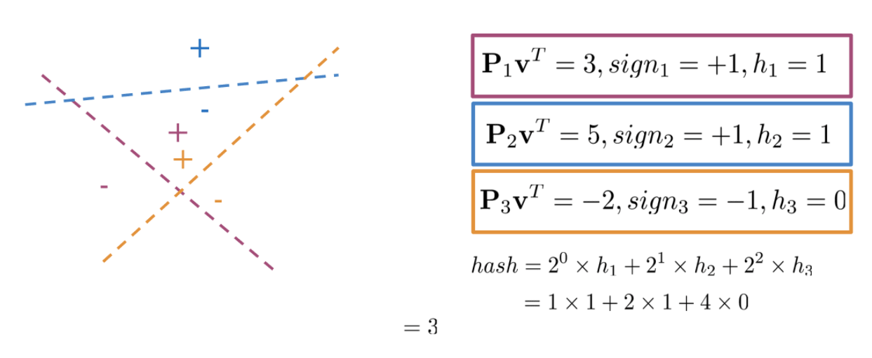
def hash_multiple_plane(P_1, V)
	"""
	return the hash of V
	"""
	hash_value=0
	for i, P in enumerate(P_1):
		sign = side_of_plane(P,V)
        hash_i =1 if sign >=0 else 0
        hash value+=2**i* hash_i
	return hash_value

Compute the hash value for Y, find the most similar vector with the same hash value.

Since the hash value depends on the planes, therefore, to get a robust result, multiple sets of random planes is used to find a combination set of neighbors.

相关图片

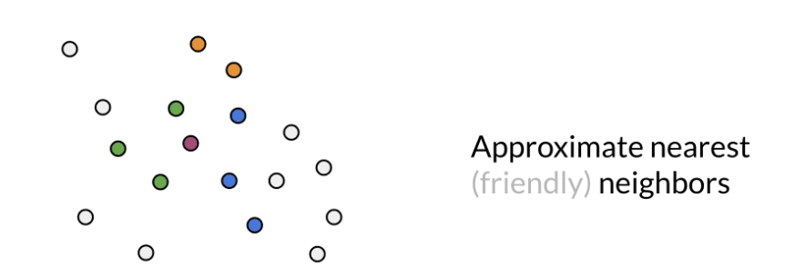
Green, blue and orange are have same hash value with rad point in different set of planes. Search the nearest point among all of them. This can be used for fast document search

Autocorrect (for misspell)

A traditional way to do autocorrect is compute the word with n edit distance and take the top-k word with high probability. To speed, a greedy method is to compute the shortest edit distance. See below. The following steps only works for misspell check.

sample code here.

STEPS

1. Identify a misspelled word

When identifying the misspelled word, you can check whether it is in the vocabulary. If you don't find it, then it is probably a typo.

2. Compute Minimum Edit distance

• Levenshtein distance: Edit cost insert 1, delete 1, replace 2

$$d\left(s_{1}, s_{2}\right)=\min\left\{\begin{array}{ll} d\left(s_{1}, s_{2}[1:]\right)+1 & \text { insert } \\ d\left(s_{1}[1:], s_{2}\right)+1 & \text { delete } \\ d\left(s_{1}[1:], s_{2}[1:]\right)+2\times\left(s_{1}[0] \neq s_{2}[0]\right) & \text { replace } \end{array}\right.$$

Algorithm:

def edit_dist(s1, s2):
    n1, n2 = len(s1), len(s2)
    d = [[0] * (n2 + 1) for _ in range(n1 + 1)]
    for i in range(n1 + 1):
        d[i][n2] = n1 - i
    for j in range(n2 + 1):
        d[n1][j] = n2 - j
    for i in range(n1 - 1, -1, -1):
        for j in range(n2 - 1, -1, -1):
            d[i][j] = min(d[i+1][j]+1, d[i][j+1]+1, d[i+1][j+1] + (s1[i] != s2[j]))
    return d[0][0]

3. Filter Candidates

4. Calculate word probabilities

$$P(w) = \frac {C(w)}{V}$$

C: Number of times word appears

V: Total size of the corpus

Pick the one with largest probability.

Part of Speech Tagging (POS tagging)

the process of assigning a part of speech to a word. All probability you used is from the corpus you collect. For the POS tagging, how you train the states and how to label the data domain the result.

Sample code here

A algorithm to generate a sequence of word given a given sentence is the Viterbi Algorithm . It compute based on the Markov Chains and Hidden Markov Models

Data Processing

data format:

相关图片

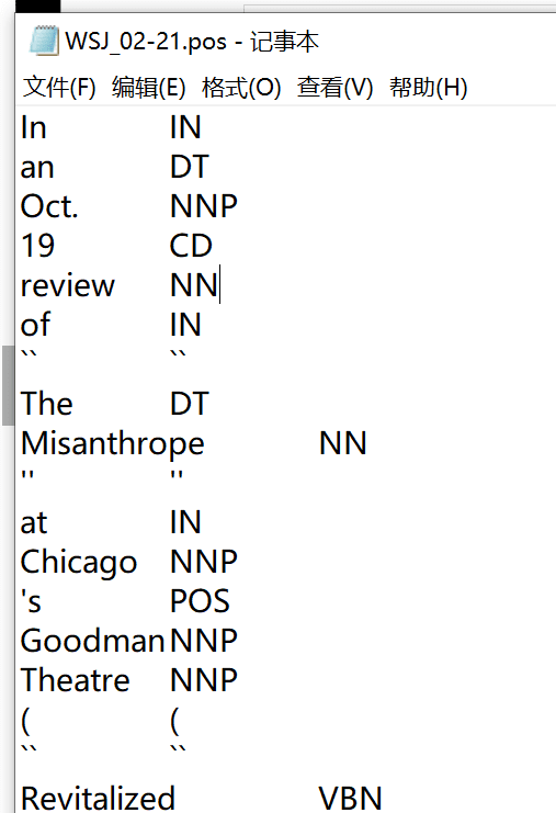
Hand labeled data, maintain the following information:

• word order
• word to tag
• start of new sentence

handling unknow words

• assign tag using suffix
• assign tag --unk--

Markov Chains

相关图片

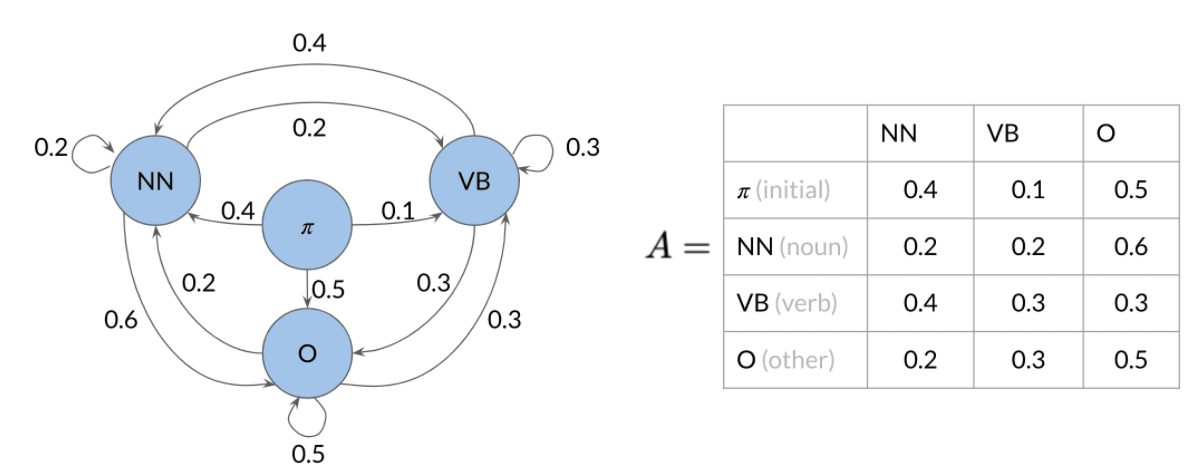
Computing the transition matrix A, Given states Q. This is based on your corpus.

Hidden Markov Models

Emission probabilities $P(w_i|t_i)$

The likelihood of a curtain each state yield a word

To get the emission probabilities:

1. Count the frequency of each word and Calculating probabilities

The $C(t_{(i-1)},t_{(i)})$ is the count of times tag (i-1) shows up before tag i.

$$P\left(t_{i} \mid t_{i-1}\right)=\frac{C\left(t_{i-1}, t_{i}\right)}{\sum_{j=1}^{N} C\left(t_{i-1}, t_{j}\right)}$$

2. Smooth and avoid 0 probability.

$$P\left(t_{i} \mid t_{i-1}\right)=\frac{C\left(t_{i-1}, t_{i}\right)+\epsilon}{\sum_{j=1}^{N} C\left(t_{i-1}, t_{j}\right)+N* \epsilon}$$

3. Computing Emission matrix

$$\begin{aligned} P\left(w_{i} \mid t_{i}\right) &=\frac{C\left(t_{i}, w_{i}\right)+\epsilon}{\sum_{j=1}^{V} C\left(t_{i}, w_{j}\right)+N * \epsilon} \\ &=\frac{C\left(t_{i}, w_{i}\right)+\epsilon}{C\left(t_{i}\right)+N * \epsilon} \end{aligned}$$

The Viterbi Algorithm

STEPS

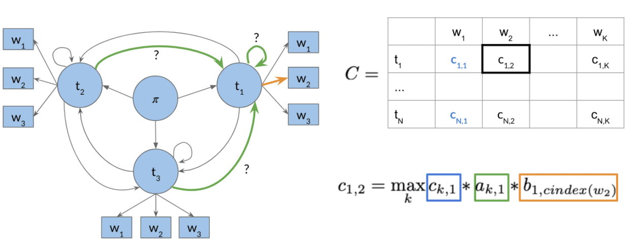
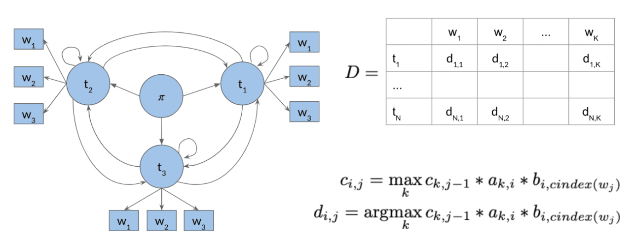
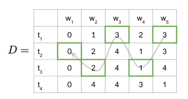
1. Initialization Probability Matrix C, previous action records: D

相关图片

相关图片

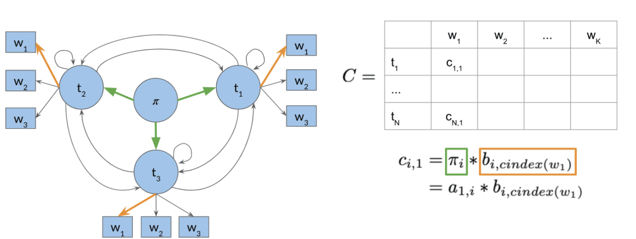
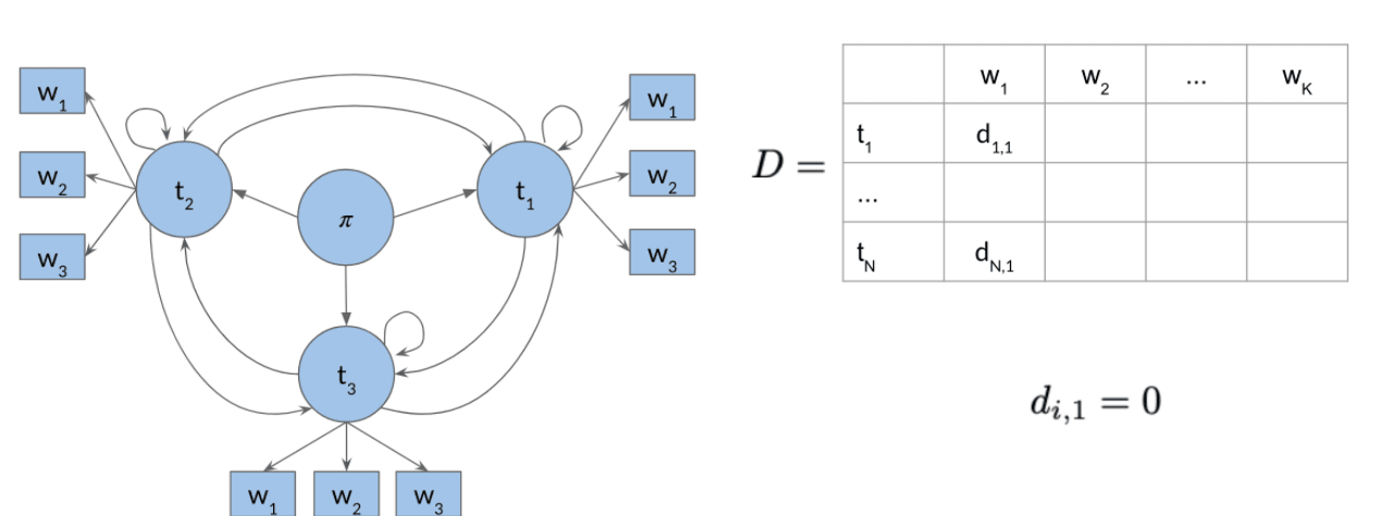
where B is the emission matrix of dimension (num_tags,len(vocab))

2. Forward pass

相关图片

相关图片

3. Backward pass

相关图片

N-grams

N-grams are fundamental and give you a foundation that will allow you to understand more complicated models in the specialization. These models allow you to calculate probabilities of certain words happening in a specific sequence. Using that, you can build an auto-correct or even a search suggestion tool.

Prefix of N-gram

padding n-1 start token if you use n gram.

Bigram

相关图片

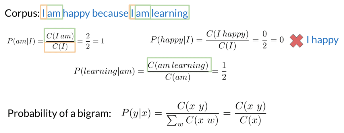
Probability of N-Grams:

$$\begin{array}{l} P\left(w_{N} \mid w_{1}^{N-1}\right)=\frac{C\left(w_{1}^{N-1} w_{N}\right)}{C\left(w_{1}^{N-1}\right)} \\ C\left(w_{1}^{N-1} w_{N}\right)=C\left(w_{1}^{N}\right) \end{array}$$

Sequence probabilities should be:

$$P(A, B, C, D)=P(A) P(B \mid A) P(C \mid A, B) P(D \mid A, B, C)$$

However, under Markov assumption: only the last n words matters the next word. we can get the approximate sequence probabilities.

$$P\left(w_{1}^{n}\right) \approx \prod_{i=1}^{n} P\left(w_{i} \mid w_{i-1}\right)$$

Starting and ending sentences <s> </s>

相关图片

相关图片

$$\begin{array}{l} P\left(w_{n} \mid w_{n-N+1}^{n-1}\right)=\frac{C\left(w_{n-}^{n-1}{N}+1, w_{n}\right)}{C\left(w_{n-N+1}^{n-1}\right)} \\ \operatorname{sum}(\text { row })=\sum_{w \in V} C\left(w_{n-N+1}^{n-1}, w\right)=C\left(w_{n-N+1}^{n-1}\right) \end{array}$$

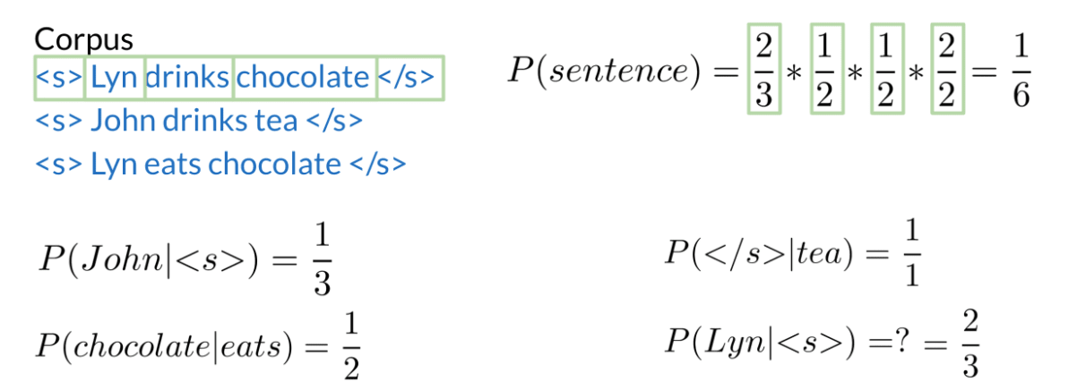
Limitation

• Large N-grams to capture dependencies between distant words
• Need a lot of space and RAM

Language Model Evaluation

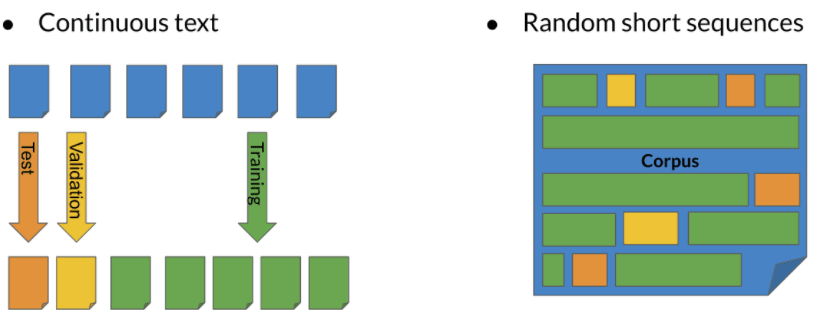
Test data split method

(8/1/1 for small corpora or 98/1/1 for large)

image-20210429155302477

Perplexity

a text that is written by human is more likely to have a lower perplexity score

$$P P(W)=P\left(s_{1}, s_{2}, \ldots, s_{m}\right)^{-\frac{1}{m}}$$

W: test set containing m sentences s The $s_i$ i-th sentence in the test set, each ending with</s> m: number of all words in entire test set W including </s> but not including <s>

$$P P(W)=\sqrt[m]{\prod_{i=1}^{m} \prod_{j=1}^{\left|s_{i}\right|} \frac{1}{P\left(w_{j}^{(i)} \mid w_{j-1}^{(i)}\right)}}$$

$$w_{j}^{(i)} \rightarrow \mathrm{j} \text { -th word in } \mathrm{i} \text { -th sentence }$$

$$P P(W)=\sqrt[m]{\prod_{i=1}^{m} \frac{1}{P\left(w_{i} \mid w_{i-1}\right)}} \quad w_{i \rightarrow \mathrm{i} \text { -th word in test set}}$$

Log perplexity:

Usually, a log PP between 4.3 - 5.9 is good.

$$\log P P(W)=-\frac{1}{m} \sum_{i=1}^{m} \log _{2}\left(P\left(w_{i} \mid w_{i-1}\right)\right)$$

def calculate_perplexity(sentence, n_gram_counts, n_plus1_gram_counts, vocabulary_size, k=1.0):
    """
    Calculate perplexity for a list of sentences
    
    Args:
        sentence: List of strings
        n_gram_counts: Dictionary of counts of n-grams
        n_plus1_gram_counts: Dictionary of counts of (n+1)-grams
        vocabulary_size: number of unique words in the vocabulary
        k: Positive smoothing constant
    
    Returns:
        Perplexity score
    """
    n = len(list(n_gram_counts.keys())[0]) 
    sentence = ["<s>"] * n + sentence + ["<e>"]
    sentence = tuple(sentence)
    N = len(sentence)
    product_pi = 1.0
    for t in range(n, N):
        n_gram = sentence[t-n:t]
        word = sentence[t]
        probability = estimate_probability(word, n_gram, 
                         n_gram_counts, n_plus1_gram_counts, vocabulary_size, k=k)
        product_pi *= probability
    perplexity = product_pi**-(1/(N))
    return perplexity

Out of Vocabulary OOV Words

• Create vocabulary V
  • Min word frequency
  • Max V size

Smoothing

4 methods to avoid N-gram probability being 0.

• Add-one smoothing (Laplacian smoothing)

this work only when vocabulary is large enough

• Add-k smoothing

$$P\left(w_{n} \mid w_{n-1}\right)=\frac{C\left(w_{n-1}, w_{n}\right)+k}{\sum_{w \in V}\left(C\left(w_{n-1}, w\right)+k\right)}=\frac{C\left(w_{n-1}, w_{n}\right)+k}{C\left(w_{n-1}\right)+k * V}$$

• bach-off
  • If N-gram missing => use (N-1)-gram, …: Using the lower level N-grams (i.e. (N-1)-gram, (N-2)-gram, down to unigram) distorts the probability distribution. Especially for smaller corpora, some probability needs to be discounted from higher level N-grams to use it for lower level N-grams.
  • Probability discounting e.g. Katz backoff: makes use of discounting.
  • “Stupid” backoff: If the higher order N-gram probability is missing, the lower order N-gram probability is used, just multiplied by a constant. A constant of about 0.4 was experimentally shown to work well
• interpolation

$$\hat{P}\left(w_{n} \mid w_{n-2} w_{n-1}\right)=\lambda_{1} \times P\left(w_{n} \mid w_{n-2} w_{n-1}\right)+\lambda_{2} \times P\left(w_{n} \mid w_{n-1}\right)+\lambda_{3} \times P\left(w_{n}\right)$$

Word Embeddings

The task to create word embedding is self-supervised : it is both unsupervised in the sense that the input data — the corpus — is unlabelled, and supervised in the sense that the data itself provides the necessary context which would ordinarily make up the labels.

Methods Overview

Classical Methods

• word2vec (Google, 2013)

• Continuous bag-of-words (CBOW)**: the model learns to predict the center word given some context words.

• Continuous skip-gram / Skip-gram with negative sampling (SGNS): the model learns to predict the words surrounding a given input word.

• Global Vectors (GloVe) (Stanford, 2014): factorizes the logarithm of the corpus's word co-occurrence matrix, similar to the count matrix you’ve used before.

• fastText (Facebook, 2016)**: based on the skip-gram model and takes into account the structure of words by representing words as an n-gram of characters. It supports out-of-vocabulary (OOV) words.

Deep learning, contextual embeddings

In these more advanced models, words have different embeddings depending on their context. You can download pre-trained embeddings for the following models.

• BERT (Google, 2018):

• ELMo (Allen Institute for AI, 2018)

• GPT-2 (OpenAI, 2018)

CBOW

STEPS:

1. Processing data: Cleaning and Tokenization

• letter case
• Punctuation
• numbers - <number>
• special characters - emojy

2. Create Training set

The concept of window size is ok to be different.

相关图片

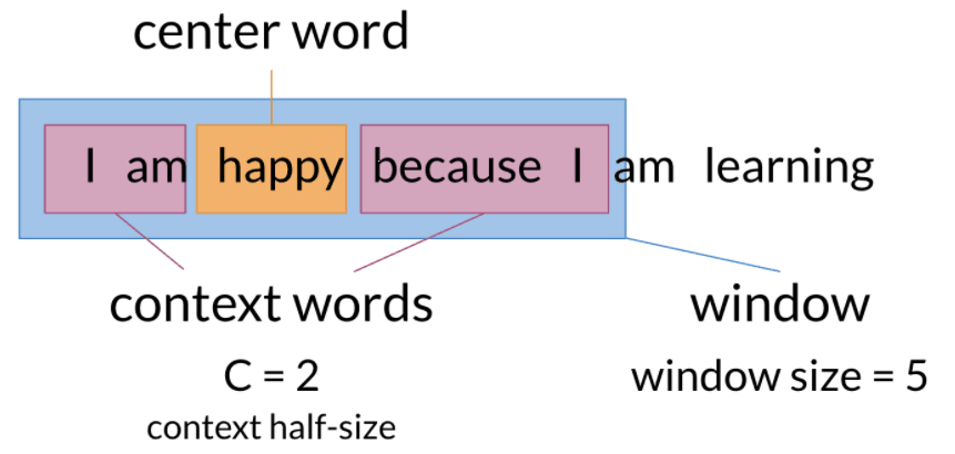
• CBOW takes the mean of context words , and used to predict the center word.
• to improve, weighted average is considered.

3. Building Model Architecture and Train

相关图片

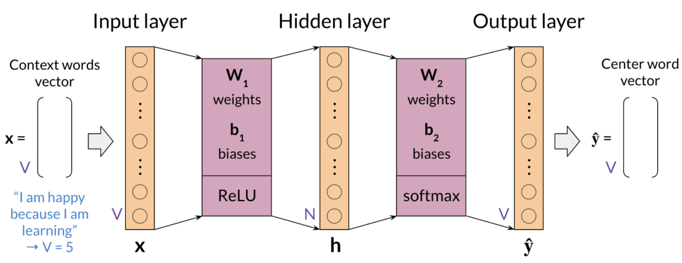
4. Extracting word embedding Vectors

3 different ways to get the word embedding

相关图片

相关图片

相关图片

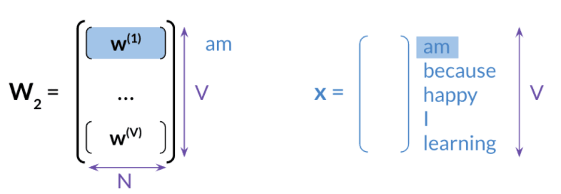
Back propagation

$$\begin{array}{l} \frac{\partial J_{\text {batch }}}{\partial \mathbf{W}_{1}}=\frac{1}{m} \operatorname{Re} L U\left(\mathbf{W}_{2}^{\top}(\hat{\mathbf{Y}}-\mathbf{Y})\right) \mathbf{X}^{\top} \\ \frac{\partial J_{\text {batch }}}{\partial \mathbf{W}_{2}}=\frac{1}{m}(\hat{\mathbf{Y}}-\mathbf{Y}) \mathbf{H}^{\top} \\ \frac{\partial J_{\text {batch }}}{\partial \mathbf{b}_{1}}=\frac{1}{m} \operatorname{Re} L U\left(\mathbf{W}_{2}^{\top}(\hat{\mathbf{Y}}-\mathbf{Y})\right) \mathbf{1}_{m}^{\top} \\ \frac{\partial J_{\text {batch }}}{\partial \mathbf{b}_{\mathbf{2}}}=\frac{1}{m}(\hat{\mathbf{Y}}-\mathbf{Y}) \mathbf{1}_{m}^{\top} \end{array}$$

Skip-Gram

STEPS

1. Cleaning and Tokenizing

which is same with CBOW

2. Getting training set

sentence: The dog barked at the mailman

相关图片

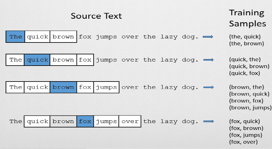
(The window size can be tune)

3. Training model

use the above training samples to train the following model. optimizing the cross entropy. the input and output word are represent as one hot vector.

相关图片

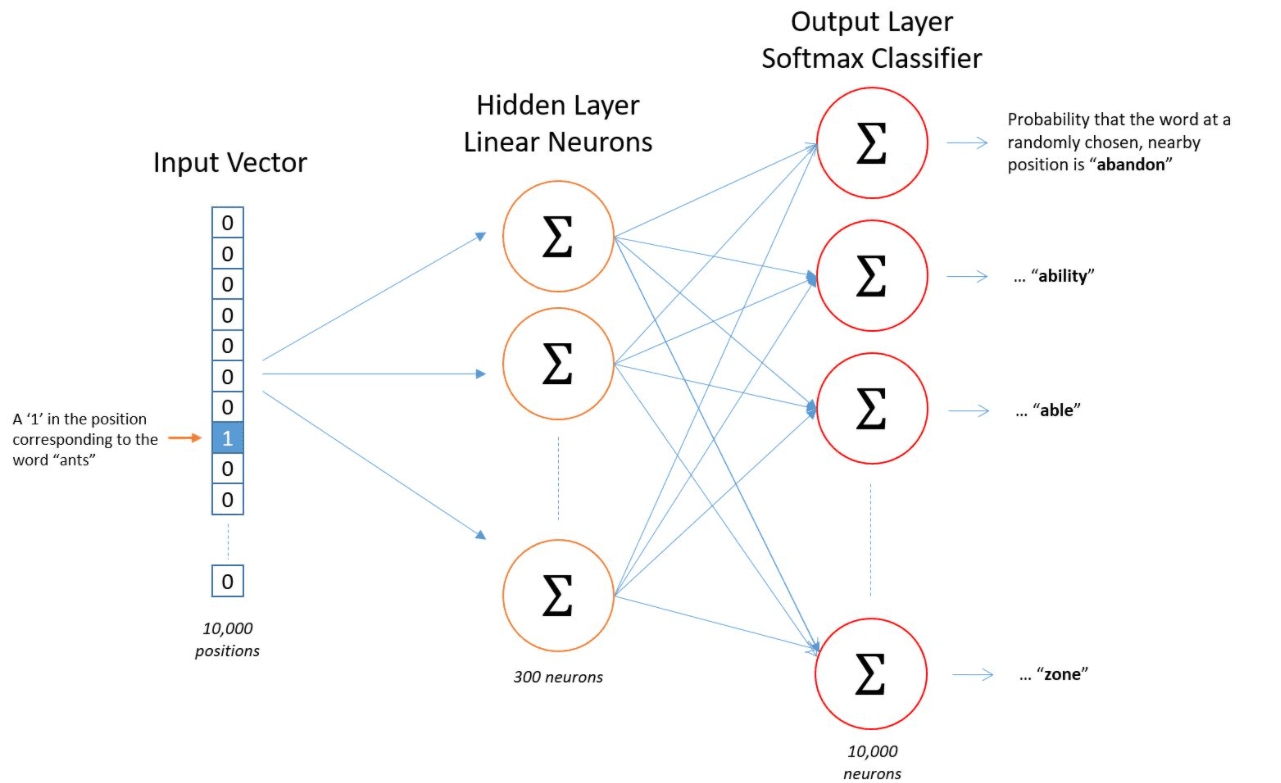
Size of hidden layer: the dimension of word vector usually being 100 to few thousand.

4. Extracting word embedding Vectors

Negative Sampling

Training set:

• one positive sample: {orange, juice}

• k negative sample: {orange, king} etc

  • k = 5-20 for smaller data sets
  • k = 2-5 for larger data set

Instead of training 10000 binary logistic classifier for the softmax layer, we are only train only 1+k samples of them.

Author recommend selecting negative examples with frequency of

$$P\left(w_{i}\right)=\frac{f\left(w_{i}\right)^{3 / 4}}{\sum_{j=0}^{n}\left(f\left(w_{j}\right)^{3 / 4}\right)}$$

Evaluating word Embeddings

Intrinsic Evaluation

• Analogies

“France” is to “Paris” as “Italy” is to ?> and also syntactic analogies as “seen” is to “saw” as “been” is to ?>.

• Clustering
• Visualization

Extrinsic Evaluation

tests word embeddings on external tasks like named entity recognition, parts-of-speech tagging, etc.

Evaluates actual usefulness of embeddings

Time-consuming

More difficult to troubleshoot

Neural Networks for Sentiment Analysis

Try different many-to-one architecture. In this sample code, a simple LSTM can perform better than the baseline model.

Hints

• Try Using Mean Layer after embedding layer

Named Entity Recognition

Named Entity Recognition (NER) locates and extracts predefined entities from text. It allows you to find places, organizations, names, time and dates.

Sample code here

Applications:

• Search engine efficiency

• Recommendation engines

• Customer service

• Automatic trading

Data Processing

• Convert words and entity classes into arrays:
• Pad with tokens: Set sequence length to a certain number and use the <PAD> token to fill empty spaces, this token key will be used to mask the array when training.

Once you have that, you can assign each class a number, and each word a number.

image-20210429213917063

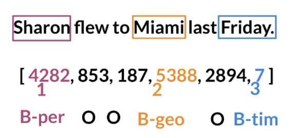
Siamese Networks

sample code

Application:

• Handwritten checks

• Question Duplicates [sample code]

• Queries

• Can do Voice checking?

Loss of siamese Networds

• Contrastive Loss
• Triplet loss Deep metric learning using Triplet network；
• Softmax loss：
• cosine loss，exp function, etc.

One Shot Learning

Compare with one shot learning, Classification got trouble when updating the classes.

STEPS

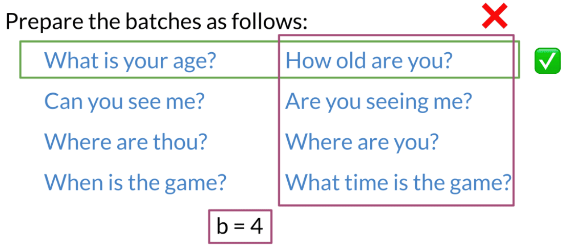
1. Prepare Batches

• Since we are going to use Hard negative mining, Sentence in the same batch should not be same meaning.
• $i_{th}$ sentence in both batch should have same meaning.

相关图片

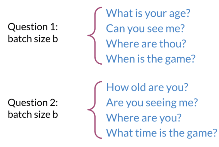
produce batches $([q1_1, q1_2, q1_3, ...]$, $[q2_1, q2_2,q2_3, ...])$ where $q1_i$ and $q2_k$ are duplicate if and only if $i = k$.

2. Build model and train

A simple Siamese Networks is shown here for learning purpose.

相关图片

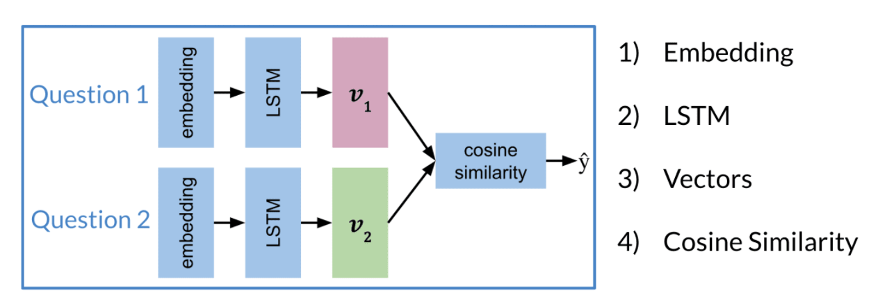
3. Testing

• The similarity of $v_1$ and $v_2$ determines the question similarity.

Hard Negative Mining

The Selection of samples determines the learning speed of the model because of the loss function we choose.

Full Cost: $max(-cos (A, P) + cos(A,N) + \alpha ,0 )$

• 𝜶: controls how far $cos(A,P)$ is from $cos(A,N)$
• Easy negative triplet, little to learn: $cos(A,N) < cos(A,P)$, the gradient will be 0.
• Semi-hard negative triplet: $cos(A,N) < cos(A,P) < cos(A,N) + \alpha$
• Hard negative triplet, more to learn: $cos(A,P) \approx cos(A,N)$

Use hard Negative Mining to avoid this problem a bit. The steps is shown in the following:

相关图片

相关图片

相关图片

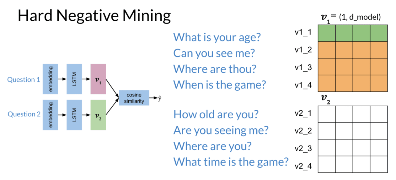
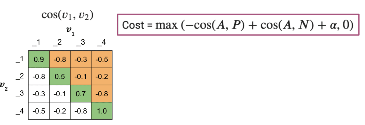
Use mean negative and closest negative cost to improve:

$$\begin{align} \mathcal{Loss_1(A,P,N)} &=\max \left( -cos(A,P) + mean_{neg} +\alpha, 0\right) \\ \mathcal{Loss_2(A,P,N)} &=\max \left( -cos(A,P) + closest_{neg} +\alpha, 0\right) \\ \mathcal{Loss(A,P,N)} &= mean(Loss_1 + Loss_2) \\ \end{align}$$

Reference

Note and Picture source: NLP specialization